Why?

While working with data, either in your traditional data science role, or performing exploratory data analysis for your machine learning task, visualizing it is an immensely important task. But creating visualizations for data that is expressed in more than three dimensions is a very difficult task.

So how can we study the relations between the different features of the data in higher dimensions?

One way would be to look at the relations pairwise, and observe their relations through a quantity known as covariance:

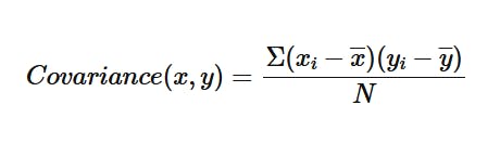
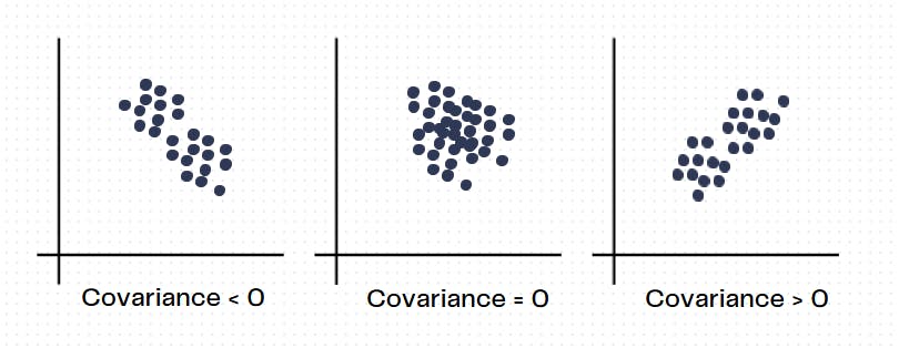
This quantity measures the relationship between two variables, and to what extent they vary together. It considers the spread of the data of both variables and tries to find the linear correlation between the two. Covariance can be either:

• Positive - This implies that both the variables show similar behavior and the increase of one value of one quantity, corresponds to an increase in the values of the other quantity.

• Negative - This implies that both variables show an inverse relationship. In this sense, when one quantity increases, the other one decreases.

If the covariance between two quantities is very close to zero, it means that they don't have a linear relation between them.

This analysis can work fine for small sets of data with let's say, 5 or 6 features. But since there are N*(N-1)/2 pairs for N features, the number scales up quickly. For N = 50 features, there will be 1225 covariance plots.

Also, sometimes there are feature pairs that have a non-linear relationship, which we can't understand through covariance plots. Finally, maybe you want to look at the spread of data, while taking into account three, four, or more features. In this case, covariance isn't sufficient for our needs.

This is where principal component analysis comes into the picture!

What?

Principal Component Analysis, better known as PCA, is a widely used technique in statistics that is used to reduce the dimensionality of a dataset while retaining as much information (variance or spread) of the data as possible. In machine learning, it's known as an unsupervised algorithm that can learn or generate its principal components, without any sort of labeled data.

PCA uses the power of Linear Algebra to find a lower-dimensional subspace (composed of principal components), such that the dataset, from the higher dimension, can be projected onto this subspace, while still keeping its patterns within the data intact.

The projected data can be used to feed into machine learning algorithms, and decrease the computation time (sometimes very significantly), making the data much easier to process.

How?

There are majorly five steps involved in this process. We will have a look at them one by one:

Step 1: Standardizing Variables

Data obtained from various sources will rarely be in the same range. Some features may range from 0 to 3, while others range from -100 to 1000, the possibilities are endless really.

To have less skewed data, and improve the performance of machine learning algorithms such as gradient descent, we will scale the data. This scaling of data can be done in two ways:

• Min-Max Scaling

• Standardization

Min-Max Scaling

We will transform each value of the feature as such:

Here, i stands for the index of the row or the data entry, and j stands for the index of the feature value in a data matrix X. If we apply this operation on all the data elements, then all our data will lie within (-1,1) . However, let's say that a feature in the data matrix had some outliers, in that case, the denominator for a particular feature would be very large. This would result in very squished, or stretched values. Usually, datasets contain outliers, therefore this method isn't always applicable. A better way to scale data would be Standardization.

Standardization

We will transform each value of the feature as such:

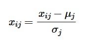
Here, similarly, i stands for the index of the row or the data entry, and j stands for the index of the feature value in a data matrix X. Upon applying this operation, to a feature column j, the values' distribution becomes closer to a Gaussian distribution. This ensures that the data is well spread and it is observed that Gradient Descent converges faster after applying this because the data becomes less skewed. We can observe this in the level curves of the loss function:

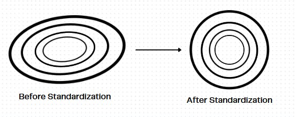
A Gaussian distribution is symmetrical about its mean. In this distribution, the mean is zero, and the standard deviation is one. Most importantly, after this transformation, even the outliers, will not create a drastic effect on the data, as the transformation is dependent on all the data points of the feature.

Now, since all the values are on the same scale we can proceed with further calculations.

Step 2: Covariance Matrix

To understand how one feature varies with another, we will use the Covariance Matrix. As we had seen earlier, we can analyze the relationship of one variable with another using covariance, here we can simultaneously see the covariance between all the pairs of features using the matrix. Therefore, the matrix contains information about the entire dataset in a way.

The Covariance matrix is a p x p matrix, where p is the number of features of the dataset. In the matrix we observe the following:

• Cov(x,x) = Var(x) - along the diagonal the covariance of a feature with itself is its variance.

• Cov(x,y) = Cov(y,x) - the covariance is symmetric in nature since the covariance quantity depends on the two features involved and not their order.

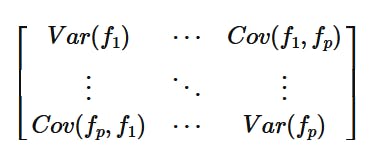
Here, f_i represents the i-th feature.

Now using this Covariance Matrix, we can obtain the principal components, such that they capture the variance of the data.

Step 3: Eigendecomposition

To find the principal components of the data, we can resort to finding out the Eigenvectors and Eigenvalues of the Covariance Matrix. Since the covariance matrix stores data about the way quantities in the dataset vary with each other, the eigenvector corresponding to the largest eigenvalue is that component that captures the highest variance. Then, the second-most largest eigenvalue's eigenvector is the second principal component.

Thus, the i-th eigenvalue's eigenvector is the i-th largest principal component, that captures the i-th most variance.

These eigenvalues and eigenvectors are obtained by solving the following equation:

$$Ax = \lambda x$$

The different values of λ give different eigenvalues, with which we can compose the eigenvectors. We can then rank the different eigenvectors based on their eigenvalues. These eigenvectors or principal components are new variables that are constructed using old ones. They have been created in such a way that they are orthogonal (that is, they have minimal correlation) and they contain the most information within themselves.

An alternate way to think about the procedure to find principal components is by first finding a line that passes through the data, which after the data is projected on it, has the maximum amount of variance (because you want to keep the most amount of patterns in the data). Then for the next component, we find a line that is perpendicular to all the previous ones (in this case the first one) and have the same objective - maximize the variance of the projected data. We continue this until we have obtained the required number of principal components. For p features, we can have at most p principal components.

If you are looking to project data in three dimensions, then you can consider the first three principal components and discard the remaining ones. Here, we can take a look at the breast cancer dataset. We can't visualize the same in its entire form because it contains a lot of dimensions, hence we must use PCA to analyze the data. We can see how the data looks with three principal components, which we can flatten further to just two principal components.

From this data, while doing PCA we calculate that:

Variance contained in:
1st principal component = 44.272025607526366%
2nd principal component = 18.971182044033082%
3rd principal component = 9.39316325743138%
4th principal component = 6.602134915470158%
5th principal component = 5.495768492346268%
6th principal component = 4.024522039883327%
7th principal component = 2.250733712976862%
8th principal component = 1.5887237999693722%
9th principal component = 1.389649374526528%
10th principal component = 1.1689781892545572%

Step 4: To keep or not to keep?

After the Eigendecomposition, we will have all the eigenvalues and their eigenvectors, we can choose which ones to keep. The matrix that contains all the principal components as its column vectors are called the feature vector. By finding out how much variance the data has, we can add them up to get the total information contained in our axes.

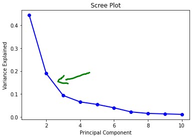
Usually, we can pick out the required eigenvectors until there is a sharp dip in the proportion of the variance contained in that principal component. This is analyzed using a scree plot.

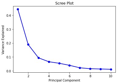
As we can see, we should consider those principal components till which there is a sharp drop in the variance, so in this case, it's the first two principal components:

Step 5: Transform data

Now that we have got the principal components. We must fit the data onto them. That is, we must project all the data along the obtained eigenvectors. After doing that, the dataset that we obtain can be used for further purposes, either visualization, or down the ML pipeline.

We can mathematically do this by using the feature vector. As the feature vector is composed of the original variables, we can compose the new dataset as such:

$$\text{Final dataset} = \text{Feature Vector}^{T} * \text{Scaled Dataset}$$

And now we are finally ready to use our dataset!

Where?

Other than in machine learning, where is PCA used? Some places are:

• Image compression - to resize the images as per the requirement

• Finance - to analyze stocks and other varying parameters quantitatively

• Recommendation Systems - to take into account all the variables that the system depends on

Conclusion

I hope you found this article useful! Feel free to suggest places for improvement!